Information Theory for Deep Learning

Despite the lack of strong theoretical bounds, Deep Neural Networks have been embarrassingly successful in various practical tasks in fields ranging from Computer Vision, Natural Language Processing, medicine, etc. There has been much work in understanding how these systems work and the community has started to view them not as black boxes.

This survey aims to study Neural Networks from an Information Theory standpoint. The majority of this survey can be viewed as the study of the ingenious work by Tishby and Schwartz-Ziv in this field and the followup critical work by Andrew M. Saxe et. al. In the end we provide some small experiments of our own which might help resolve at least some of the conflicts.

To start, we will first review the mathematical foundation required to make sense of Tishby’s findings. We will start by exploring a Deep Neural Network setting designed to solve a classification problem. This kind of a framework lies at the heart of many problems discussed above.

The input variable \(X\) here is generally a very large dimensional random variable, whereas the output variable \(Y\) (to be predicted) is not as large in dimensionality.

For instance, in ImageNet challenge 2017 the average size of an image is 482x415 pixels, which is about 200K dimensional and the output variable is only 200 in dimension. In terms of information theory, the number of bits required to represent the output variable is \(\approx\) 8 i.e. (\(log_{2} 200\)).

This means that the features in \(X\) that are informative about \(Y\) are scattered in some sense and may be difficult to extract.

Readers well versed in basic information theory may skip the next section.

Information Theory: Prerequisites

For the sections to follow, the logarithm is chosen in base 2 so that the units of the quantities talked further can be interpreted in terms of bits.

KL Divergence

KL Divergence is simply a measure of how two probability distributions differ. For discrete probability distributions \(P\) and \(Q\),

Entropy

The entropy of a discrete random variable X (taking values in {\(x_1, x_2, ... , x_n\)}), with a probability mass function \(P(X)\) is defined as:

Also we can define conditional entropy of two random variables X and Y as follows:

Mutual Information

The mutual information between two random variables (X and Y) is a quantification of the amount of information that is obtained about one random variable from the other.

Invariance to invertible transforms

For any invertible functions \(\Phi, \Psi\):

Data Processing Inequality (DPI)

For any markovian chain of random variables \(X \rightarrow T \rightarrow Y\):

DNNs form a Markov Chain

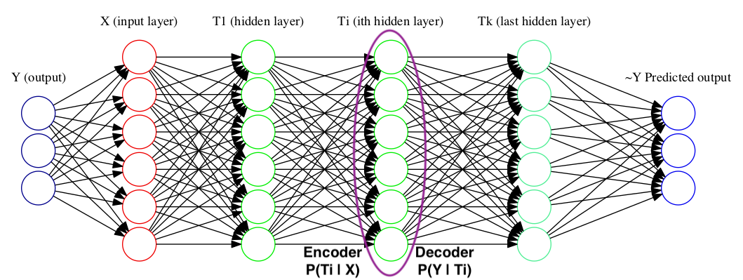
The output of each layer may be considered as a random variable \(T\), and thus is just a representation of the input random variable. Each such representation \(T\) may be defined using an encoder distribution \(P(T \lvert X)\) and \(P(\hat{Y} \lvert T)\). Such distributions may be further used to describe \(I_X = I(X;T)\) and \(I_Y = I(T;Y)\). Collectively, plotting \(I_X\), \(I_Y\) over time(during training) for different layers can help us understand the dynamics of what actually happens during training.

By the data processing inequality we have:

These two set of inequalities tell us that the plot of \(I_X\) vs \(I_Y\) will be monotonically increasing as we move from the predicted variable to the input variable. (across the layers)

Information Bottleneck applied to understand DNNs

Any DNN, given the set of input and output and a predefined learning task, tries to learn some representation \(T\) of \(X\) which characterized \(Y\). What might be a good enough representation? One such representation is the minimal sufficient statistic. Tishby et al. 1999, gave an optimization problem which gives an approximate sufficient statistic. This framework represents the tradeoff between the compression of the input variable \(X\) and the prediction of \(Y\).

For a markov chain \(Y \rightarrow X \rightarrow X \rightarrow T \rightarrow \hat{Y}\), with probability distributions \(p(t \lvert x), p(t), p(y \lvert t)\) minimize:

This objective is easy to look at using the following argument. Think of the first term trying to compress the input and the second term is trying to retain only that information relevant for \(Y\). Thereby this framework squeezes out the information from \(X\) relevant to only \(Y\).

Further, \(I(X;T)\) corresponds to the learning complexity and \(I(T;Y)\) corresponds to test/generalization error.

Now the idea is to utilize this curve and study how the information plane of DNN looks with respect to such an information bottleneck framework.

The original idea of the ‘Opening the black box of Deep Neural Networks via Information’ paper by Tishby et al. 2017 is to:

Demonstrate the effectiveness of the visualization of DNNs in the information plane for a better understating of the training dynamics, learning processes, and internal representations in Deep Learning (DL).

Experimental setup

Their idea involves plotting the information plane(traced by the DNNs during training with SGD) and the information bottleneck curve which represents the limit. So this experiment will involve knowing the joint probability distribution of the data beforehand. Also, the mutual information of discrete random variables will have to be estimated by knowing only a handful of samples from the entire data distribution, but how to do that is reserved for a later post.

SGD Layer Dynamics in Info Plane

The reader is encouraged to view the video above which clearly shows how the information plane evolves over time (over epochs) and across the layers which is shown by dots in different colors. There are many dots of one color which simply represent the different initialization states over the neural network.

If we look at the last layer (the dots in orange) it is evident that they show a behaviour which is constantly increasing in the \(Y\) axis, but shows a convex behaviour in \(X\) axis, ie. it first increases with respect to \(X\) and reaches a maximum (at around 400 epochs) followed by a final decrease in the \(X\) axis.

This behavior is explained by the author as a distinct two-stage process which involves:

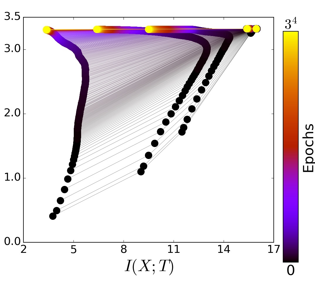
1. Fast ERM stage This phase is characterized by the steep increase of \(I_Y\). Also, this fast stage takes only some hundred epochs out of the total 10K iterations in the example data set.
2. Slow Training phase (Representation compression phase) The second stage is much longer and in fact, takes up most of the time that is more than 9K epochs out of the total. During this phase, the information \(I(X;T)\) decreases for each layer (though this loss is more prominent for the later layers, DPI is respected) and all non-essential information of \(X\) with respect to \(Y\) is essentially lost.

Drift and Diffusion

The discussion above is from the standpoint of the information plane. Another interesting viewpoint of the training dynamics of neural networks is observed if the same timeline of epochs is observed with the evolution of weights. That is the mean and standard deviation of weights for a particular layer is tracked over the course of training.

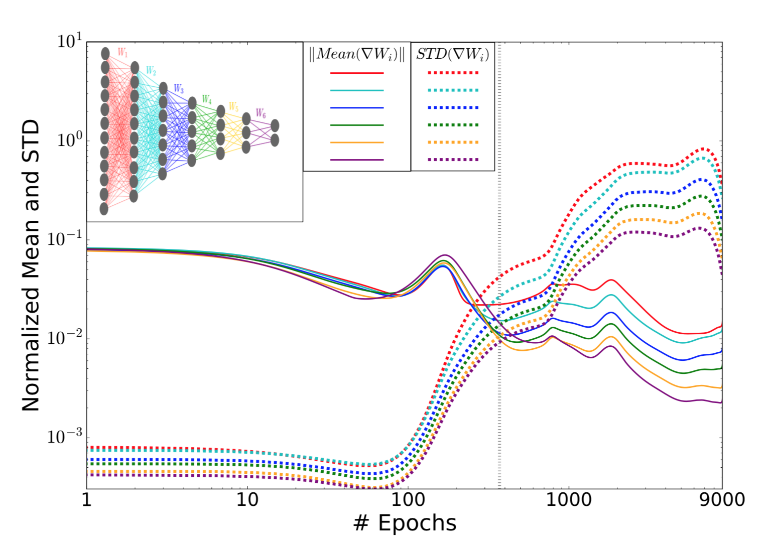
The first phase is characterized by weights which have high mean and small variance, and thus a small SNR. This phase is called the drift phase and denotes small stochasticity. Similarly, the second phase is when the SNR is relatively larger and so the gradients act like noise (sampled from a Gaussian distribution with a very small mean) to each of the layers and is called the diffusion phase by the authors.

We see that there is a significant jerk in the SNR of the weights at around 400 epochs. Notice the clear two distinct phases observed in this evolution too! In fact, the epoch at which this marked change is observed is the same at which we begin to see the compression behavior beginning in the information plane. This points to the fact that there is a causal relation between SGD dynamics and the generalization performance.

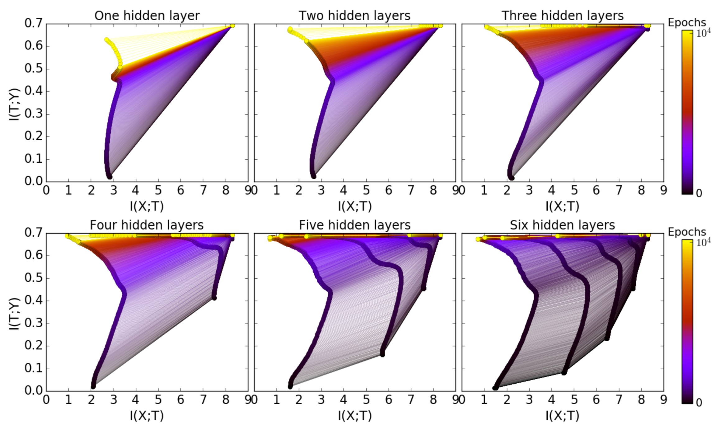
Hidden Layers

The authors have empirically shown using some experiments that there is computational benefit by adding more hidden layers and the same can be verified by the image included below.

1. The number of training epochs is reduced for good generalization.
2. Compression phase of each layer is shorter.
3. The compression is faster for layers close to the output.

Optimal IB representation

To test if the trained network actually closely satisfies the optimal information bottleneck objective the authors conducted the following experiment. Using the already calculated values of \(p(t \lvert x)\) and \(p(y \lvert t)\) they then apply the framework of information bottleneck to calculate the optimal \(p_{\beta}^{IB} (t \lvert x)\). This uses the ith layer decoder, \(p(y \lvert t)\) and any given value of \(\beta\).

Then for each layer, they calculated the optimal \(\beta^{*}\) by minimizing the average distance between the optimal IB decoder distribution and the ith layer encoder.

Further, they plot the IB information curve (theoretical) and then mark the actual values of \(I_X\) and \(I_Y\) for the different layers of the neural network on this same plot.

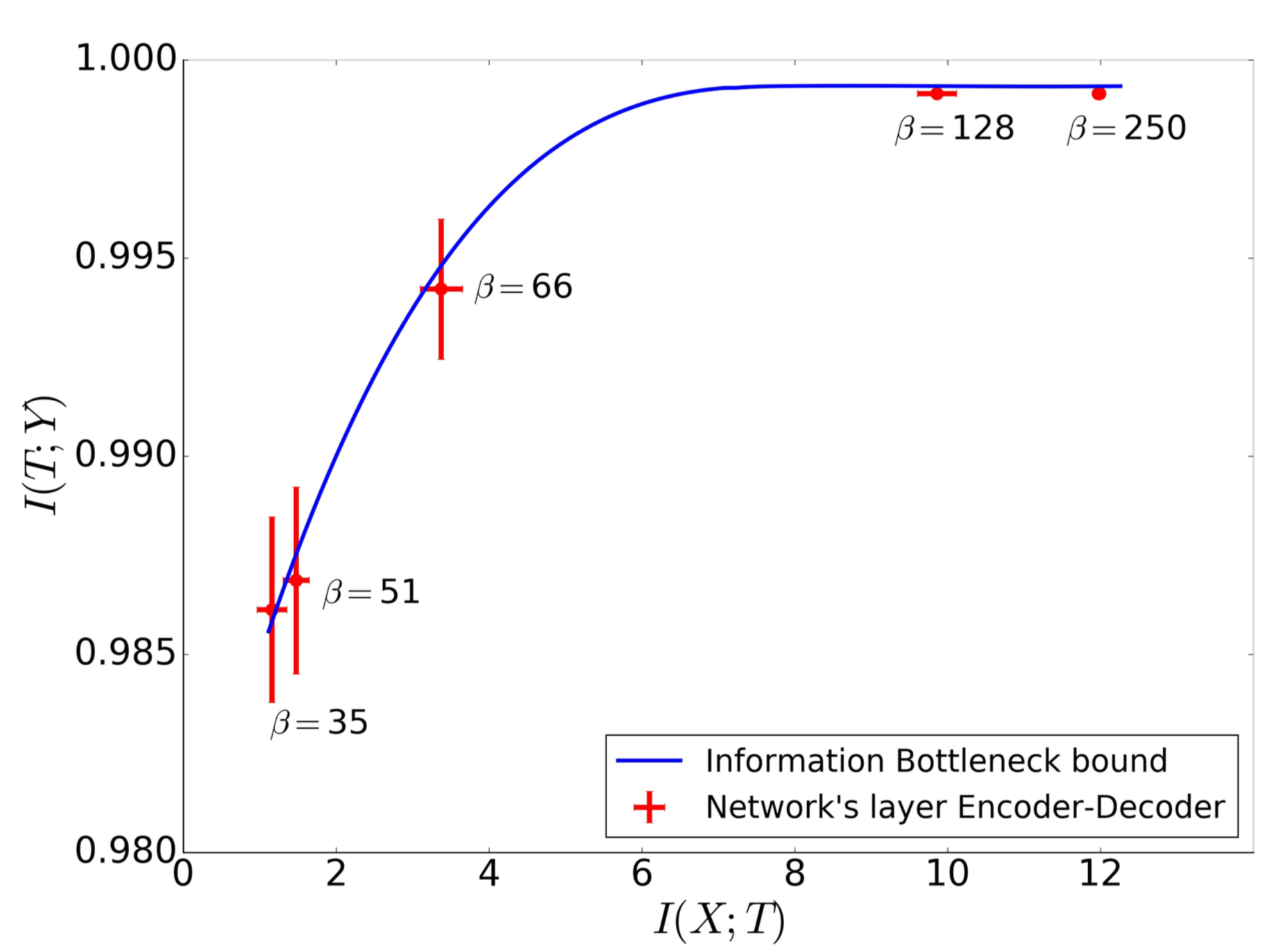
Viola, the slope of the curve at the points \(I_X\) and \(I_Y\) for the different layers should be \(\beta^{-1}\) which lies incredibly close to the calculated optimal \(\beta^{*}\) for each layer. This points to the fact that the DNNs actually capture an optimal IB representation.

New Generalization bounds for Neural Networks

The authors state that the training of a neural network comprises of two stages - fitting and compression and the excellent generalization performance of deep networks is attributed to the latter.

In his recent seminar at Stanford, Naftaly Tishby attempts to prove that compression leads to a dramatic improvement in generalization.

He proposes to reconsider learning theory for deep neural networks based on his belief that the existing generalization bounds are too weak for Deep Learning.

Earlier Generalization Bounds

Here,
\(\epsilon\) is the generalization error
\(\delta\) is the confidence
\(m\) is the number of training examples
\(H_{\epsilon}\) is the \(\epsilon\) cover of the Hypothesis class

\(\lvert H_{\epsilon} \rvert\) is typically assumed to be \(\lvert H_{\epsilon} \rvert \approx \left(\frac{1}{\epsilon}\right)^d\)
with \(d\) being the complexity (Rademacher complexity, VC dimension, etc) of the Hypothesis class

Although these bounds guide researchers on how much of generalization is possible for most of the problems, these bounds are quite vacuous for deep learning as the VC dimension of deep neural networks is of the order of the number of parameters and neural networks work surprisingly well for datasets much smaller than the number of parameters.

Tishby proposes generalization bounds based on input compression which he believes to be tighter as compared to the earlier generalization bounds.

Tighter Input Compression Bounds proposed by Tishby

According to the Shannon McMillan limit for entropy,

\[H(x) = - \lim_{n \rightarrow \infty} \frac{1}{n} \log p(x_1, …, x_n)\]

With most of the inputs \(X = x_1, …, x_n\) being typical with probability:

\[p(x_1, …, x_n) = 2^{- n H(X)}\]

Similarly, for partitions \(T\) that are typical and are large enough,

\[p(x_1, …, x_n \vert T) = 2^{- n H(X \vert T)}\]

According to the earlier generalization bounds, \(\epsilon^2 < \frac{\log \lvert H_{\epsilon} \rvert + \log 1 / \delta}{2m}\) where \(\lvert H_{\epsilon} \rvert \approx \left(\frac{1}{\epsilon}\right)^d\)

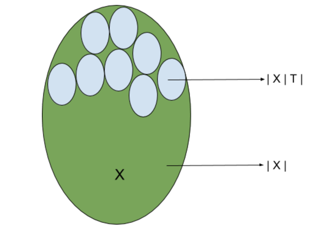
However, given the above idea, \(\lvert H_{\epsilon} \rvert\) can be approximated as \(\lvert H_{\epsilon} \rvert \approx 2^{\lvert T_{\epsilon} \rvert}\)

where \(T_{\epsilon}\) is the \(\epsilon\) partition of the input variable \(X\).

\(\lvert T_{\epsilon} \rvert \approx \frac{\lvert X \rvert}{\lvert X \vert T_{\epsilon} \rvert}\) provided that the partitions remain homogenous to the label probability.

With the above assumption, the Shannon McMillan limit results in

\[\lvert T_{\epsilon} \rvert \approx \frac{2^{H(X)}}{2^{H(X \vert T_{\epsilon})}} = 2^{I( T_{\epsilon}; X)}\]

Thus we have the following generalization bound based on input compression as proposed by Tishby

\[\epsilon^2 < \frac{2^{I( T_{\epsilon}; X)} + \log 1 / \delta}{2m}\]

This generalization bound depends on \(I( T_{\epsilon}; X)\) and decreases when the information between \(T_{\epsilon}\) and \(X\) reduces.

\(K\) bits of compression of the input reduces the training examples requirement by a factor of \(2^K\) if this bound applies and is tight. Thus, a bit of compression is as effective as doubling the size of the training data.

The authors argue that compression is necessary for good generalization error and hence justify the compression phase of neural network training.

Critical Response by Andrew M. Saxe et al

Saxe et al present a critical review of Tishby et al’s explanation of deep learning success through their information compression arguments. They present their opposition to the three specific claims made by Tishby et al.

Claim 1: Distinct fitting and compression phases

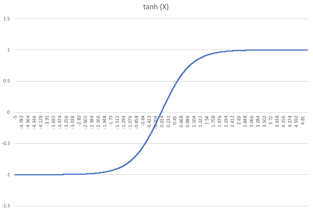
The authors argue that compression or loss in mutual information between the hidden layers and the input arises primarily due to saturation of the non-linear activations used and is related to the assumption of binning of noise in the hidden layer representation.

Tishby et al had made use of the \(\tanh\) (hyperbolic tangent) function as the activation function. The \(\tanh\) function saturates to 1 and -1 on high positive and negative values respectively. Saxe et al claim that compression achieved by Tishby et al was due to the fact that \(\tanh\) is a double saturating function, i.e. it saturates on both the sides and binning such a function results in a non-invertible mapping between the input and the hidden layer. For large weights, the \(\tanh\) hidden unit almost always saturates yielding a discrete variable concentrating in just two bins. This lowers the mutual information between the hidden unit and the input to just 1 bit.

As the weights tend to increase during training, they are forced to concentrate into a smaller number of bins to which the authors attribute the reason for the compression phase as was observed by the original authors.

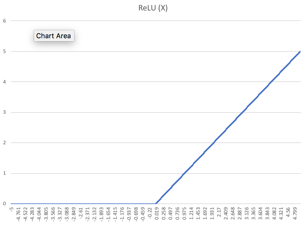
To test this notion, Saxe et al repeat the same procedure for \(ReLU\) with all the layers containing \(ReLU\) units except for the final output layer containing sigmoid units. The authors report no apparent compression phase for \(ReLU\) units.

The authors justify their observations by noting that \(ReLU\) is a single saturating function. With \(ReLU\) nonlinearity, inputs are no longer forced to concentrate into a limited number of bins even for large weights as the positive half of \(ReLU\) is a linear function.

The authors also provide an exact mathematical proof of how the entropy reduces for larger weights in the case of \(\tanh\) nonlinearity but not in the case of the \(ReLU\) non-linearity through a simple example consisting of a single hidden layer with a single neuron with a single input and output.

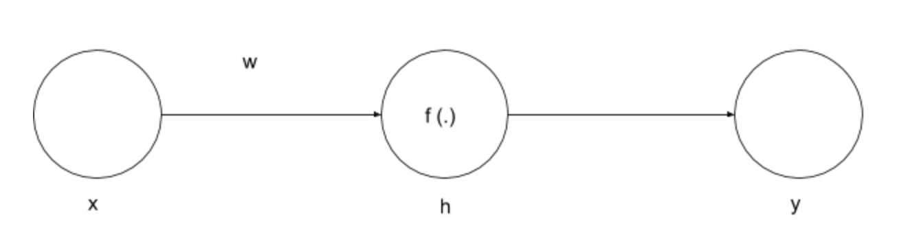
This network has a single input \(X\) and output \(Y\). The hidden layer \(h\) is binned yielding a new discrete variable \(T = bin(h)\). Here, the mutual information between \(T\) and \(X\) is calculated as

\[I(T; X) = H(T) - H(T \vert X) = H(T) = - \sum_{i = 0}^N p_i \log p_i\]

where \(p_i = P (h \geq b_i \text{ and } h < b_{i + 1})\) is the probability that the hidden unit activity \(h\) produced by input \(X\) is binned to bin \(i\). For monotonic non-linearities, this can be rewritten as

\[p_i = P (X \geq f^{-1}(b_i) / w \text{ and } X < f^{-1}(b_{i + 1}) / w)\]

The following graphs show entropy of \(T\) or its mutual information with input \(X\) as a function of weights for an input arriving from a uniform distribution.

The above graphs show that the mutual information with the input decreases as a function of the weights after increasing first for the \(\tanh\) non-linearity but increases monotonically for the \(ReLU\) non-linearity.

An intuitive way to understand the above result is that for very large weights, the \(\tanh\) hidden unit saturates yielding a discrete variable that concentrates primarily in just two bins, the lowest and the highest bin leading to the mutual information with the input of just one bit.

Saxe et al attribute the compression phase of neural network training as advocated by Tishby et al to the information compression due to binning for double saturating non-linearities as shown above.

Thus, the new authors attempt to refute the claim of the existence of distinct fitting and compression phases made by the original authors.

Claim 2: The excellent generalization of deep networks due to the compression phase

The authors claim that there exists no causal connection between compression and generalization. In other words, networks that do not compress are still capable of generalization and vice-versa.

In their argument against the previous claim, the authors portrayed the role of non-linearity in the observed compression behavior and attributing it to double saturating non-linearities and the binning methodology used to compute mutual information. However even without non-linearity, neurons could converge to highly correlated activations, or discard irrelevant information from the input as in the case of deep linear networks Baldi and Hornik (1989), Fukumizu (1998) and Saxe et al. (2014).

The authors use simple linear networks trained in a student-teacher setting where the “student” neural network is fed with the output of the teacher neural network and the student learns. In recent results by Advani and Saxe,2017 it has been shown that this setting generates a data set which allows for generalization performance calculation, exact computation of the mutual information (without any sort of quantization) and a direct computation of the IB bound.

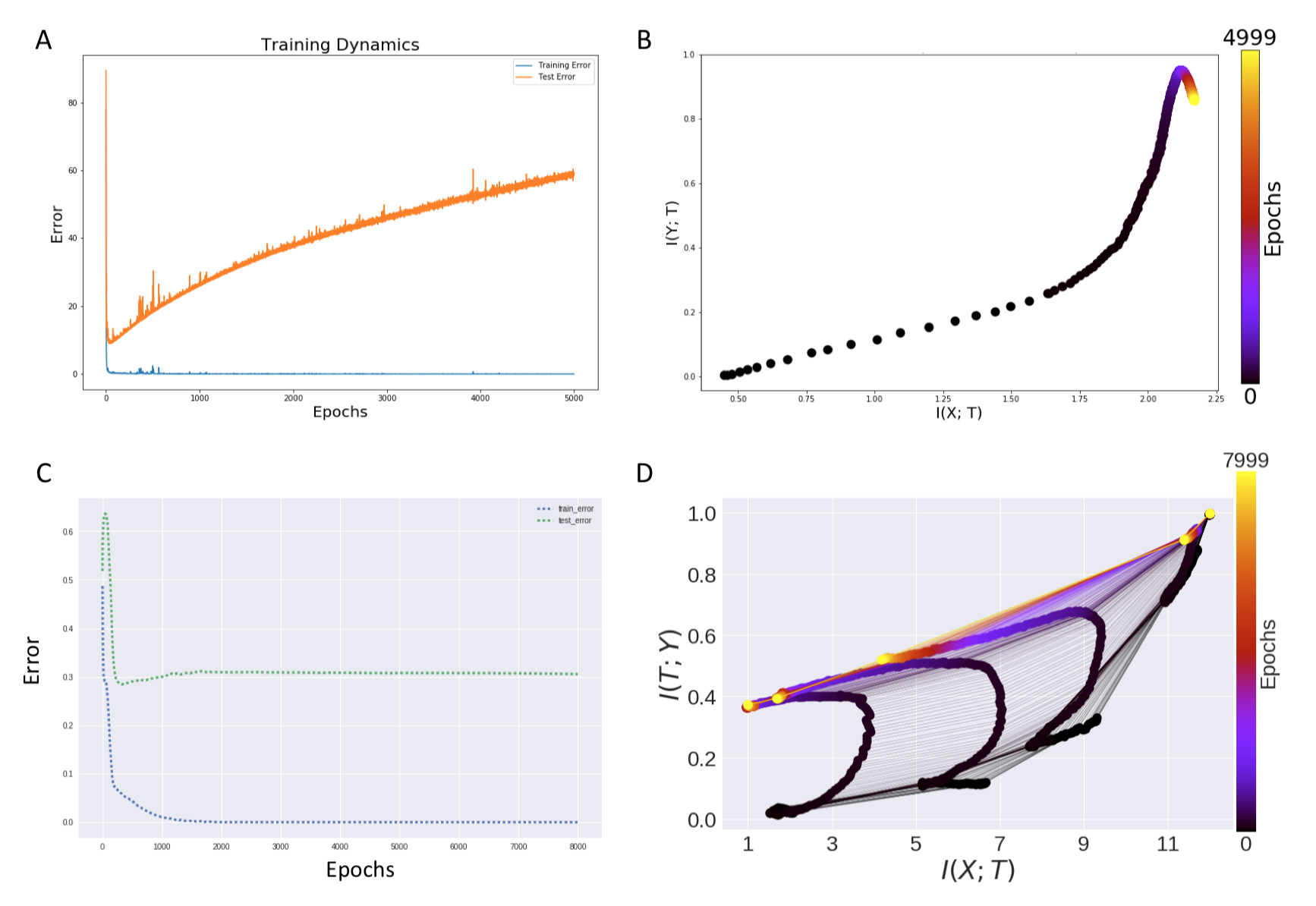
Next, the authors show using this setup that even with networks where it is known that they generalize well over data, compression might not be possible. Also they show the other side of the story, i.e. with networks that overfit too much might also possibly show no compression (as seen in the above image). Thus they challenge the causality between compression and generalization bounds.

It is important to note here that the original authors had showed through their input compression bound described here that compression reduces the upper bound of the generalization error. However, the authors claim here that the original authors have not provided any rigorous argument for why it is safe to assume that deep networks result in partitions homogenous to the label probability. The information compression bound is not valid unless it can be shown that the partitions remain more or less homogenous to the label probability. We discuss further about it later by designing a simple experiment which gives a deeper insight in this matter of debate.

The authors report that they observe similar generalization performance between \(\tanh\) and \(ReLU\) networks despite different compression dynamics. Even if the bound shown by the original authors may exist, it may still be too weak. In other words, compression may not be a major factor behind the observed behavior.

Claim 3: Compression phase occurs due to diffusion - like behavior of SGD

The authors note that the compression phase, even when it exists, does not arise from stochasticity in training (one of the major results of Tishby et al.). They show this by replicating the information bottleneck findings using the full batch gradient descent and observing compression without the need for any stochasticity that was earlier originating from the stochastic gradient descent.

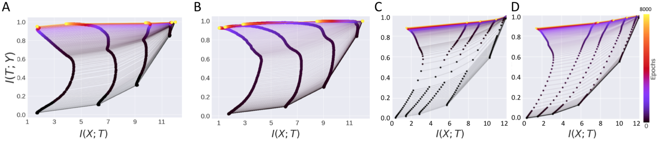
Here the figure represents four scenarios (A). \(\tanh\) network trained with SGD. (B) \(\tanh\) network trained with BGD. (C) \(ReLU\) network trained with SGD. (D) \(ReLU\) network trained with BGD. Essentially the authors provide counterexamples to the explanation that compression is attributable to SGD, by showing that Batch gradient descent shows similar information plane dynamics.

Apart from the above evidence, the authors also provide a theoretical argument for concluding the possibility for an observed compression phase without training stochasticity. Their major concern is that the distribution of weights driven to a maximum entropy constrained to the training error by the diffusion phase reflects stochasticity of weights across different training runs. The entropy of the inputs given the hidden layer activity, \(H(X \vert T)\) need not be maximized by the weights in a particular training run.

Additional Experiments for verification (!)

To resolve this debate, we propose some experiments that may be used further by researchers in this domain to establish if not completely but to some extent what might be going on this debate for the DL and the Information theory community.

Setup

We sampled uniformly data \(X\) from a set which contains all possible permutations of 4 boolean variables. So the distinct number of samples \(X\) can be at most \(2^4\) which is 16. Next the task constructed was a simple task defined as: \(y_i = ( x_{i1} \text{and } x_{i2} ) \text{ or } ( x_{i3} \text{and } x_{i4} )\)

To further complicate this task, a noise term was added to the output i.e., y was inverted (logically) with a probability of 0.07 for all samples.

The number of data points sampled using the above scheme was set to 4096 and the neural network was chosen to have hidden layers of tanh nonlinearity and the design of the layers was: Input-4-4-4-4-2-Output.

The network was trained using cross entropy loss with an SGD solver using a batch size of 16.

We have only tested these experiments on toy/small data sets but firmly believe that these experiments can be extended to real-life data sets and models and can establish at least empirically these two arguments. The entire code for this experiment is available at github.

If Neural Networks provide partitions which are homogeneous to class label probabilities

The outputs of the second last layer were pulled out and thus T (the second last layer) was analyzed for information content and partition homogeneity. This was achieved by finding an \(\epsilon\) partition over T for a particular \(\epsilon\).

In general, this problem of finding the partition is computationally hard.

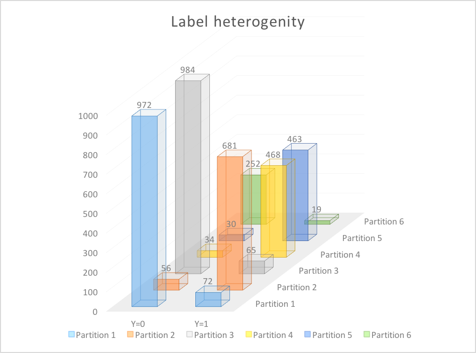
Next, we studied how the inputs were distributed among these partitions and tried to analyze if these partitions are homogeneous to label probability.

The number of partitions achieved was 6 and the total input data points was 4096 and the number of output classes was 2 as the output \(Y\) was either 0 or 1. We found that the partitions were far from homogeneous among class labels, in fact, the distributions of our findings are plotted below.

The information theoretic generalization bound is too loose

The general schema which may be used as further experimentation is provided. Essentially, we want to verify numerically how tight the bound is on generalization error in terms of the “information” quantities.

First, some synthetic data will have to be created. (We need to know the sample distribution to calculate the entropy this input data, in general, other real-life data may be utilized, but the entropy will then have to be estimated).

The next stage will involve training a neural network model with the given training data (skipping all forms of regularization, and also any tricks you might have up your sleeve including batch normalization, dropout, etc). This model will be used to calculate the difference in the test and the training error to give a numerical estimate for the generalization performance. Let us call this number \(\epsilon\). Now using the same training data and the model trained above we will compute the \(\epsilon\) partition of any hidden layer of the network.

Given such a partition and the entropy of the initial data, we can compute the mutual information of the partition given the data. This experiment may be repeated several times to give us an accurate measure of the confidence parameter which then can be finally used to show at least numerically how well this generalization bound fares.

As another fun idea, one can track the weights learnt from the network during the end of each epoch and see if the start of the compression phase aligns with the point where the current weights lead to maximized input entropy for the \(\tanh\) activation as can be seen in the entropy-weight graph.

References

[1]. Shwartz-Ziv, Ravid, and Naftali Tishby. “Opening the black box of deep neural networks via information.” arXiv preprint arXiv:1703.00810 (2017).

[2]. Saxe, A. M., Bansal, Y., Dapello, J., Advani, M., Kolchinsky, A., Tracey, B. D., and Cox, D. D. (2018). On the information bottleneck theory of deep learning. In International Conference on Learning Representations.

[3]. Tishby, Naftali, and Noga Zaslavsky. “Deep learning and the information bottleneck principle.” Information Theory Workshop (ITW), 2015 IEEE. IEEE, 2015.

[4]. Tishby, Naftali, Fernando C. Pereira, and William Bialek. “The information bottleneck method.” arXiv preprint physics/0004057 (2000).

[5]. Achille, Alessandro, and Stefano Soatto. “On the emergence of invariance and disentangling in deep representations.” arXiv preprint arXiv:1706.01350 (2017).

[6]. Advani, Madhu S., and Andrew M. Saxe. “High-dimensional dynamics of generalization error in neural networks.” arXiv preprint arXiv:1710.03667 (2017).

[7]. Poggio, Tomaso, et al. “Why and when can deep-but not shallow-networks avoid the curse of dimensionality: A review.” International Journal of Automation and Computing 14.5 (2017): 503-519.

[8]. P. Baldi and K. Hornik. Neural networks and principal component analysis: Learning from examples without local minima. Neural Networks, 2:53–58, 1989

[9]. K. Fukumizu. Effect of Batch Learning In Multilayer Neural Networks. In Proceedings of the 5th International Conference on Neural Information Processing, pp. 67–70, 1998

[10]. A.M. Saxe, J.L. McClelland, and S. Ganguli. Exact solutions to the nonlinear dynamics of learning in deep linear neural networks. In the International Conference on Learning Representations, 2014